flowchart LR
  A["analysis.Rmd<br/>(text + code chunks)"] -- "Knit" --> B{{"R runs<br/>every chunk"}}
  B --> C["analysis.html<br/>(text + code + results)"]
1 R, RStudio, and R Markdown
NoteLearning objectives
By the end of this chapter you should be able to:
- Explain how R, RStudio, and R Markdown differ, and how they fit together.
- Find your way around the four panes of RStudio.
- Create, run, and knit an R Markdown document.
- Read basic R code: lines, blocks, variables, comments, and functions.
Every chapter after this one asks you to do spatial data science: download data, clean it, analyze it, and map it. You will do all of that by writing code. This chapter introduces the three tools you will use for every lab and assignment, and the small vocabulary you need to read and write your first lines of R.
The three tools are easy to mix up, so it helps to keep one sentence in mind from the start: R is the language, RStudio is the workspace, and R Markdown is the document format. The first half of the chapter takes each in turn. The second half covers the building blocks of code that appear in every script you will write.
1.1 What is R?
R is a programming language and free software environment for statistical computing and graphics. It was created by statisticians, and its strengths still reflect that: cleaning, analyzing, modeling, and visualizing data. Statisticians, data scientists, and geographers all use it for the same reason. A few lines of R can do what would take dozens of clicks in a spreadsheet or a desktop GIS, and those lines can be run again tomorrow.
On its own, R knows how to do arithmetic, statistics, and basic plots. What makes it useful for geography is its packages (also called libraries): bundles of code, written by other users, that add new abilities. There are thousands of them. In this course you will use sf for vector data such as points, lines, and polygons, terra for rasters, tidyverse for cleaning and reshaping data, and tmap and ggplot2 for maps.
1.1.1 Why use R?
R has four strengths that make it the tool for this course.
- Power. R has a huge range of tools for statistics, machine learning, and spatial analysis, and new methods often appear as R packages before they appear anywhere else.
- Visualization. R makes high-quality, fully customizable plots, charts, and maps. Every figure in this book was made in R.
- Reproducibility. A script records every step of an analysis, so you, a classmate, or a reviewer can rerun it and check the result.
- Community. A large, global community of users builds packages, answers questions, and writes tutorials. When you get stuck, someone has almost always asked the same question online.
Reproducibility matters most for us. A point-and-click GIS workflow is hard to repeat exactly: which tool did you run, with which settings, in which order? An R script answers all of those questions in writing. When the data are updated, or when you find a mistake in step two of ten, you fix it and run the script again, and every later step updates with it.
There are practical reasons, too. R is free and open source, so everything you learn here keeps working after you graduate, with no license fees. It is updated frequently, it is popular in both research and industry, and it is consistently ranked among the most widely used languages for statistics and data analysis. The skills transfer to jobs and to graduate research.
1.2 What is RStudio?
You can type R commands into a plain window, but almost nobody works that way. RStudio is an integrated development environment (IDE) for R: one window where you write code, run it, see the results, and check your data. A good way to think about the relationship is that R is the engine and RStudio is the dashboard. R does the computing underneath; RStudio is where you work.
Because RStudio drives R, you need both, and you must install R first, then RStudio. RStudio cannot run any code until R is installed. Both are free. Installation steps are in Section 1.6 at the end of this chapter.
1.2.1 The four panes
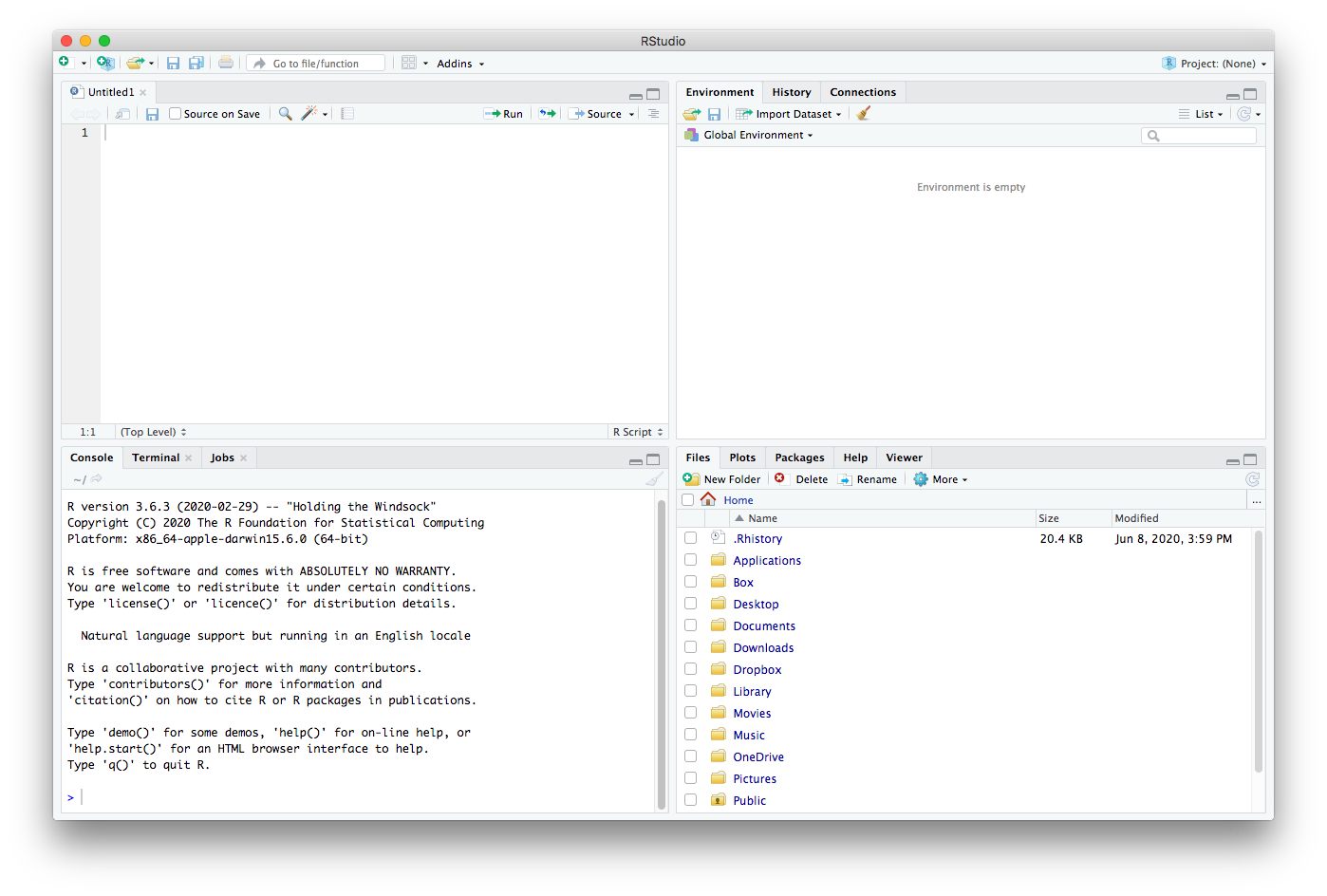
When you open RStudio, the window is divided into four panes (Figure 1.1).
| Pane | Default position | What it is for |
|---|---|---|
| Editor | Top left | Writing and saving scripts and R Markdown files |
| Console | Bottom left | Running commands and reading results, warnings, and errors |
| Environment | Top right | Listing the variables and data currently in memory |
| Files, Plots, Help | Bottom right | Browsing folders, viewing graphs, and reading documentation |
The difference between the Editor and the Console is the most important one in Table 1.1. The Editor is where your work is saved. Anything you type there can be kept in a file and run again. The Console is for quick tests: R runs a command the moment you press Enter, but nothing you type there is saved. A useful habit is to experiment in the Console and keep what works in the Editor.
The Environment pane lists every variable you have created, with a short description of what it holds. It is the first place to look when you are debugging: if a variable you expected is missing, or holds something unexpected, the Environment will show it. The bottom-right pane holds several tabs, including Files, Plots, Packages, and Help.
1.2.2 RStudio during a working session
Figure 1.2 shows RStudio partway through an analysis, with every pane in use.
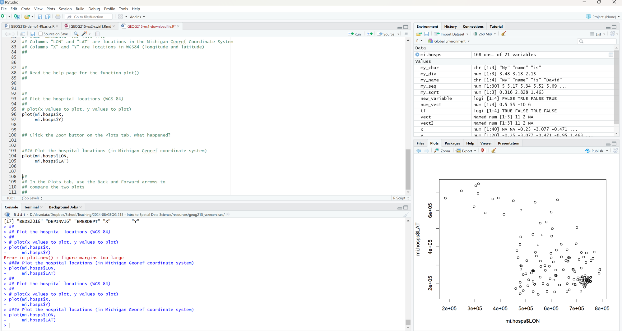
The screenshot captures the loop you will repeat constantly:
- Write a line of code in the Editor.
- Run it. Click Run, or press Ctrl+Enter (Cmd+Return on a Mac), to send the current line to the Console.
- Check the Environment. If the line created a variable, it appears there.
- Read the Console. Output, warnings, and errors print here.
- Look at the Plots pane if the line drew a graph.
Notice the red error message in the Console of Figure 1.2. Errors are a normal part of writing code, and they are not something to skip past. Read them. They usually say what went wrong, and often where. (This one, “figure margins too large,” just means the Plots pane was too small to draw the graph, and it went away when the pane was enlarged.)
1.3 R scripts and R Markdown
There are two kinds of files you will write R in, and it is worth being clear about the difference (Table 1.2).
| R script | R Markdown | |
|---|---|---|
| File extension | .R |
.Rmd |
| Contains | Code only | Formatted text with code chunks |
| Notes and explanation | Comments that start with # |
Ordinary text, headings, and lists |
| Produces | Results in the Console and Plots pane | A finished document in HTML, PDF, or Word |
| Best for | Short tasks and reusable code | Reports, labs, and assignments |
An R script is only code. Anything in it that is not code has to be written as a comment. An R Markdown file mixes formatted text and code, so the explanation of an analysis lives right next to the analysis itself. It is easier to read and easier to share. All assignments in this course are R Markdown files, so you will write both kinds of content: prose in Markdown and code inside chunks.
1.3.1 What is R Markdown?
R Markdown is a file format for dynamic, reproducible documents. An .Rmd file combines text written in Markdown, a simple way of formatting plain text, with chunks of R code. When you knit the file, R runs every code chunk and places the results (numbers, tables, and plots) into a finished document, as HTML, PDF, or Word (Figure 1.3).
The key idea is that the document and the analysis are the same file. If the data change, you knit again, and every number and figure in the report updates with them. Nothing has to be copied and pasted by hand, so nothing can fall out of date. In this course we mostly knit to HTML, because it is fastest and needs no extra software.
TipR Markdown and Quarto
This book is written in Quarto, the newer successor to R Markdown, made by the same developers. Quarto files end in .qmd instead of .Rmd, but the YAML header, Markdown text, and code chunks work the same way. Everything in this chapter applies to both.
1.3.2 Anatomy of an R Markdown file
Every R Markdown file has three kinds of content: a YAML header, Markdown text, and code chunks.
The YAML header sits at the very top of the file, between two lines of exactly three dashes. It holds metadata, which is data about data. Here it describes the document rather than the analysis: its title, author, date, and output format.
---
title: "My First R Markdown Document"
author: "Jane Doe"
date: "August 14, 2025"
output: html_document
---
R reads the header to know what to put at the top of the report and what kind of document to produce. YAML is picky: the dashes must be exactly three, each line needs a space after the colon, and indentation matters.
Markdown text is plain text with a few simple formatting marks. A line that starts with # becomes a heading (## a smaller heading, ### smaller still). Wrapping a word in single asterisks makes it italic, and double asterisks make it bold. A line that starts with - becomes an item in a bulleted list.
Code chunks hold R code. A chunk starts with three backticks followed by {r}, and ends with three backticks:
```{r}
1 + 2 + 3
```
The {r} tells R Markdown that the chunk contains R code. Click the small green “play” arrow at the top right of a chunk to run just that chunk. When the file is knit, the result prints directly below the chunk in the report:
1 + 2 + 3
#> [1] 6
The [1] in front of the answer is R’s way of saying “this is the first element of the result.” You will see it in front of almost every result R prints, and you can ignore it for now.
Putting the three pieces together, a complete (very short) R Markdown file looks like this:
---
title: "Lab 1"
author: "Jane Doe"
output: html_document
---

## How many months are in a century?

There are 12 months in a year and 100 years in a century.

```{r}
# Months in a century
months <- 12
years <- 100
months * years
```

So a century has **1,200** months.
1.3.3 The R Markdown workflow
You will follow the same four steps for every assignment.
- Create a file. In RStudio, choose File > New File > R Markdown…, give the document a title, and click OK. RStudio opens a new file that already contains a YAML header and some example content.
- Edit the document. Write your narrative in Markdown, and insert code chunks where you need them (Code > Insert Chunk, or Ctrl+Alt+I; Cmd+Option+I on a Mac).
- Run code chunks as you go, by clicking each chunk’s green play arrow, to check that each one does what you expect.
- Knit the document. Click Knit in the Editor toolbar. R builds an HTML report with all of your text, code, output, and plots, and opens it in a preview window.
Knitting does something important that is easy to miss: it reruns all of your code, from the top, in a fresh R session that knows nothing about what you have already run. A file that knits successfully is therefore a file that anyone can reproduce from scratch. If it fails to knit, the error message names the chunk that broke.
1.3.4 Keep all course files in one folder
Most of the errors students run into early in the semester are not really coding errors. They are file path errors: R cannot find a data file because the .Rmd file and the data are saved in different places. When you knit, R looks for files relative to the folder where the .Rmd file is saved, so a tidy folder structure prevents a whole category of “file not found” errors.
Create one folder for the class, called geog215, and save all of your work there, with subfolders for data, labs, and notes:
geog215/
├── data/
├── labs/
│   └── lab01.Rmd
└── notes/
Use short file names with no spaces, such as lab01.Rmd. Spaces and special characters in file names cause trouble in code, and a consistent naming pattern makes files easy to find.
1.4 Code basics
The rest of this chapter introduces five ideas that appear in every R script: lines, blocks, variables, comments, and functions. A cooking analogy runs through all of them (Table 1.3).
| Code | Cooking analogy |
|---|---|
| A line of code | One step in a recipe |
| A block of code | A recipe: several steps that make one dish |
| A program | A full meal: several recipes combined |
| A function | An appliance: ingredients go in, a dish comes out |
The code boxes in the rest of this chapter are live. Click Run Code to run the R inside them, right here in your browser. You can also edit the code and run it again, which is the best way to learn what each piece does. The first time you run a box, R takes a few seconds to load.
1.4.1 A line of code
Every program starts with one line of code, and every line does something. When you run a line, R evaluates it and returns the result. Try it:
R returns 11, again with [1] in front to mark the first element of the result. A single line is like a single step in a recipe: “chop the onion,” or “add 5 and 6.”
Sometimes a line produces no visible result. Storing a value in a variable, which you will see below, prints nothing at all. The line still did something, though. It changed what R is holding in memory.
1.4.2 A block of code
A block of code is a sequence of lines that work together on one related task, the way the steps of a recipe work together to make one dish. In an R Markdown file, a block usually lives in one code chunk. Here is a block that answers a question: how many months are in a century?
The block stores 12 in months, stores 100 in years, multiplies them, and prints the answer, 1200. Its first line starts with #, which makes it a comment, covered below.
1.4.3 Variables
A variable is a named piece of memory that holds data. Once a value is stored in a variable, you can reuse it by name instead of typing it again.
You store a value with the assignment operator, <-, which looks like an arrow pointing left. The value on the right is stored in the name on the left. Read it out loud as “gets”: months <- 12 is “months gets 12.” In RStudio, the shortcut Alt+- (Option+- on a Mac) types the arrow for you.
Variable names are case-sensitive: Months and months are two different variables. Run this box, which asks for Months with a capital M:
R replies with an error, object 'Months' not found, because no variable has exactly that name. This is one of the most common errors you will see, and now you know how to read it. Change Months to months and run the box again.
When you run code in RStudio, each new variable appears in the Environment pane. Checking that pane after you run a line is a good way to confirm that the line did what you meant.
1.4.5 Functions
A function takes inputs, does a job, and returns an output. The inputs are called arguments, and they go inside parentheses after the function’s name. If variables are the nouns of R, functions are the verbs.
In the cooking analogy, a function is an appliance, such as an oven. To make a pizza, you put bread, cheese, and tomato sauce into the oven, and the oven returns a pizza (Figure 1.4).
flowchart LR
  A["bread"] --> D{{"bake()"}}
  B["cheese"] --> D
  C["tomato_sauce"] --> D
  D --> E["pizza"]
In R, that would be written:
pizza <- bake(bread, cheese, tomato_sauce)Here bake() is the function; bread, cheese, and tomato_sauce are the arguments; and the result is stored in a new variable, pizza. (bake() isn’t a real R function, but the pattern is exactly the one every real function follows.)
R comes with hundreds of real functions, and packages add thousands more. Run this box to try a few:
c() is itself a function: it combines values into a vector, a sequence of values that R stores together. mean() and max() each take a vector and return one number. The last line converts the average to degrees Celsius. It nests one function inside another, so mean() runs first and round() rounds its result, and it shows a named argument, digits = 1, which tells round() how many decimal places to keep. Every function has a help page that lists its arguments; type ?round in the Console to see one in the Help pane.
1.4.6 Chaining functions with the pipe
Nested functions like the last line above are read from the inside out, which gets hard to follow as they grow. The pipe operator, |>, lets you write the same steps from left to right instead. The pipe takes the result on its left and passes it as the first argument to the function on its right:
This gives the same answer as round(sqrt(max(temps)), digits = 1), but reads in the order the steps happen. Read the pipe out loud as “and then”: take temps, and then find the maximum, and then take its square root, and then round it to one decimal place. You will use the pipe constantly in later chapters to string together steps that clean, analyze, and map data, and it is required in the course’s assignments.
1.4.7 A program
A program is a set of lines and blocks of code that work together to do a task, the way several recipes combine into a full meal. Every assignment in this course is a program: an R Markdown file that loads data, analyzes it, and makes a map.
R runs a program from top to bottom, so order matters. A variable must be created before it is used. When you work interactively, it is easy to run chunks out of order, or to delete a line that created a variable that is still sitting in your Environment. Everything seems to work until you knit, and then the fresh session that knitting starts in reports object not found. That error is doing you a favor: it means your file, as written, would not have worked for anyone else either.
1.5 Some hints for coding
Two habits make the biggest difference when you start writing code.
Think about the syntax. R is exact. Spelling, capital letters, commas, quotation marks, and brackets all have to be right, and every opening parenthesis needs a closing one. A single missing comma is enough to stop a program. When something fails, check the syntax of the line the error points to first.
Think about the purpose. Before you type a line, say in plain words what it should do: “store the number of years,” “find the average temperature.” If you can’t say it, you aren’t ready to write it yet. If you can, the words make a good comment.
And leave lots of comments. They are notes to Future You, who will not remember, three weeks from now, why you wrote that line.
1.6 Setting up R and RStudio
Before the first lab, set up your computer:
- Install R from CRAN, https://cran.r-project.org. Choose the download for your operating system (Windows, macOS, or Linux) and run the installer with its default settings.
- Install RStudio Desktop from Posit, https://posit.co/download/rstudio-desktop/. Remember the order: R first, then RStudio.
- Create your
geog215folder, withdata,labs, andnotessubfolders, somewhere you will find it easily. - Test everything. Open RStudio, create a new R Markdown file (File > New File > R Markdown…), save it in
geog215/labs, and click Knit. If an HTML report appears, you are ready.
1.7 Check your understanding
Which program does the actual computing when you run code: R or RStudio?
In which RStudio pane would you look to see the variables currently in memory?
What file extension does an R Markdown document have?
After running
months <- 12andyears <- 100, what doesmonths * years / 10return?Which character starts a comment in R?
In
round(3.14159, digits = 2), what isdigits = 2?True or false: knitting runs your code in a fresh R session, so a variable you created only in the Console will not exist.
months * years is 1200. Dividing by 10 gives the answer.
1.8 Summary
- R is the language that does the computing. RStudio is the workspace where you write and run R. R Markdown is the document format that combines your writing with your code and its results.
- RStudio has four panes: the Editor for writing and saving code, the Console for running commands and reading output, the Environment for the variables in memory, and Files, Plots, and Help.
- An R Markdown file has a YAML header, Markdown text, and code chunks. Knitting reruns every chunk from the top in a fresh session and builds a finished report, which is what makes the work reproducible.
- A line of code does one thing; a block of lines does one task; a program combines blocks to do a whole job, and runs from top to bottom.
- Variables store values with
<-and are case-sensitive. Comments start with#and are notes for people. Functions take arguments and return an output, and the pipe|>chains them from left to right. - Keep all course files in one folder, mind your syntax, and comment generously.
1.9 Exercises
Your first R Markdown file. Create a new R Markdown file titled “Exercise 1” with your name as the author. Delete the example content below the YAML header, add a heading, and write one sentence about why you are taking this course. Knit it to HTML.
Arithmetic. In a code chunk, calculate how many hours are in a year, and how many seconds. Store each intermediate value (days, hours per day, and so on) in a variable with a clear name, and add a comment to each line.
Read the error. Run each line below, one at a time, in the Console, and explain in your own words what is wrong. Two of them give an error message. The first gives a
+prompt instead: what is R waiting for? (Press Esc to get back to the normal>prompt.)mean(c(1, 2, 3) Mean(c(1, 2, 3)) mean(c(1, 2 3))Functions and help. Look up the help page for
seq()with?seq. Use it to create the sequence 0, 5, 10, …, 100, and store it in a variable. Then uselength(),sum(), andmean()on your variable.Nesting versus piping. Rewrite
round(sqrt(sum(c(4, 9, 16))), 2)using the pipe|>. Check that both versions give the same result.Order matters. Write a chunk that uses a variable before it is created, and knit the file. What happens? Fix the chunk so that the file knits.
1.10 Further reading
- R for Data Science by Hadley Wickham, Mine Çetinkaya-Rundel, and Garrett Grolemund is free online at https://r4ds.hadley.nz. Its early chapters cover the RStudio workflow, the basics of R code, and the pipe in more depth.
- R Markdown: The Definitive Guide by Yihui Xie, J. J. Allaire, and Garrett Grolemund, free at https://bookdown.org/yihui/rmarkdown/, is the full reference for R Markdown.
- In RStudio, Help > Cheat Sheets links to one-page summaries of the RStudio IDE and R Markdown that are worth printing and keeping by your computer.
1.4.4 Comments
A comment is a note for people, not for R. A comment begins with
#, and R ignores everything after the#on that line. In the century example above, R skipped# How many months are in a century?, but a reader knows straight away what the block is for.Use comments to explain why your code does what it does, not just what it does. The code itself already says that
months * yearsmultiplies two numbers. A good comment says why you needed that number. When you return to an assignment weeks later, comments are what let you understand your own reasoning, and in this course they are also how your instructor sees it.