Background
In this brief tutorial, we’ll examine machine learning through multi-class classification in the Dzetsaka classification plugin in QGIS. Dzetsaka was written by Nicolas Karasiak. The Dzetsaka plugin works in QGIS to take raster (often satellite imagery) data and uses a set of training data to build land type classifications. Traditionally, the tool was developed to determine different types of vegetation in the landscape, although it works well (with training and validation) on different types of land covers.
Land cover refers to visible categories of land use in a given area. These could include:
- Tree cover (high coverage >80%, medium coverage, low coverage)
- Water
- Built-up areas
- Grassland
- Settlements / homes
- Shrub
- Bare soil
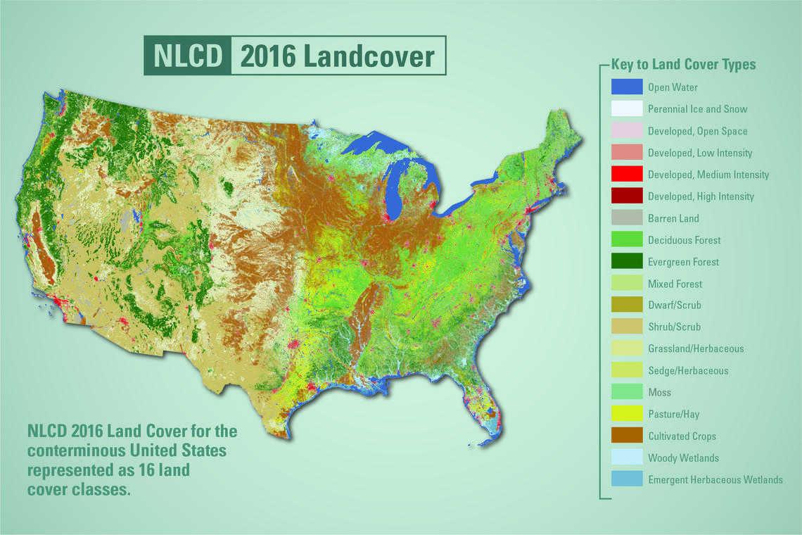
The types of land cover you choose will be up to you, depending on the area you’re classifying. In this example, we’ll be using a high-resolution orthoimage from the USGS EROS Archive at USGS’s EarthExplorer.
This tutorial covers the following steps:
- Background
- Installation
- Preparation
- Building Region Classes
- Classifying using Training
- Smoothing and Vectorizing the Results
- Validating the Model
- Next Steps
Installation
Install QGIS
If you haven’t installed QGIS, please download and install QGIS on your Windows, Mac, or Linux computer. The Dzetsaka plugin should work with recent versions of QGIS.
Install scikit-learn
Before running QGIS, be sure to have the scikit-learn Python module installed in your QGIS path. To do this, follow one of these methods:
☐ On Windows, open the OSGeo4W Shell and run
python3 - m pip install scikit-learn -U --user
☐ On linux and Mac, open a shell and run
python3 - m pip install scikit-learn -U --userInstalling the dzetsaka plugin
☐ Open QGIS, open the Plugins menu and select Manage and Install Plugins.☐ Search for dzetsaka and choose Install Plugin.

Preparation
For this tutorial, I’ve prepared a data set ready to use. You can, of course, substitute your own files and the process will largely be the same.
☐ Download this zip folder, and extract the data into a folder you can access.
☐ To open the project, double-click on the machine-learning.qgz file.
The data consists of the following files:
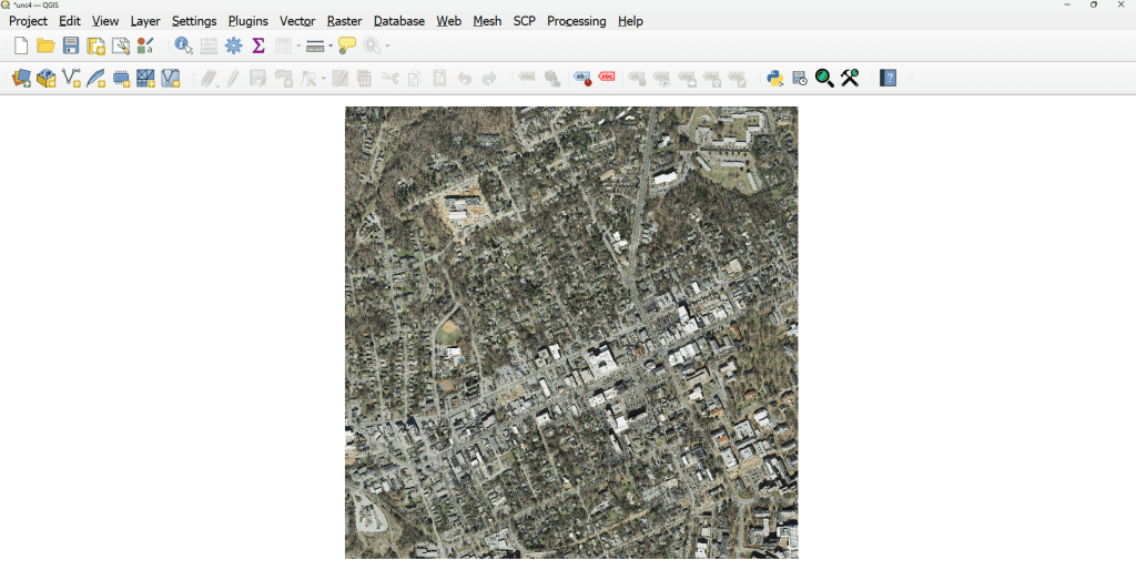
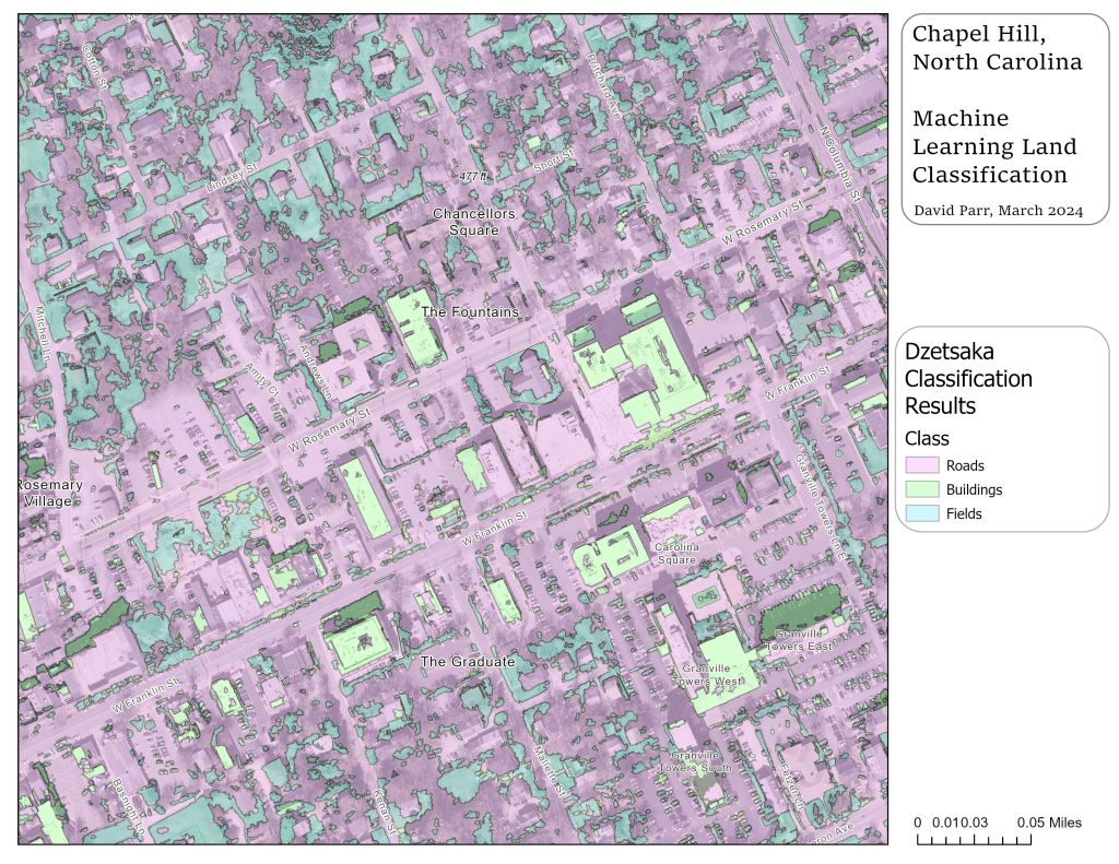
- oc6iO_37_000_10978801_20130220_0304r0.tif – a 3-band corrected orthoimage of Chapel Hill, NC from February 20, 2013.
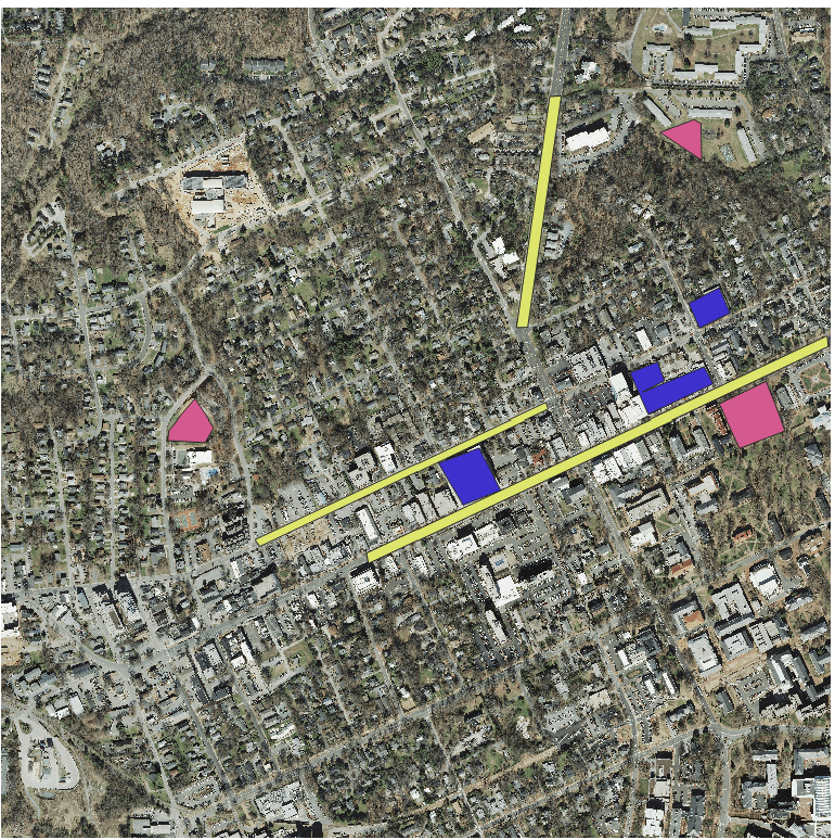
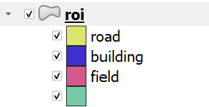
- A prepared roi.shp (Region of Interest) shapefile with three land cover types: roads, buildings, and fields. This file will hold our training data.
- An example output raster (out.tif) from an earlier run.
- An example smoothed raster (sieve.tif) from an earlier run.
- And an example vectorized, classified shapefile (vectorized.shp) from an earlier run.
All of the data is the tutorial is in the EPSG:2264, NAD83 / North Carolina (ftUS) projection. The cell size of the raster is .5 feet. It’s important that you keep your projection consistent between data and appropriate for the location that you’re running analysis on.
NOTE: If you haven’t extracted the data from the zip folder, it may not appear in QGIS. Be sure to extract the data.
Building Region Classes
The sample data includes a Region of Interest file (roi.shp) that has predefined classes in the data. These are meant to help train the classifier in progress. You can modify / add / remove these training data and classes.
Modifying the Training Data Classes
The classes in the roi file are defined in an attribute called class. Class itself is an integer attribute in a Value Map which adds an associated label.
☐ To modify the class types, right click on the roi layer and go to Properties.
☐ Under Properties, go to Attribute Form, and click on the class Field to access the Widget Type.
☐ Add / modify / remove values in the Value/Description box. Be sure that each class has a unique numerical value.

Changing the classes of your training data may make sense depending on the area you’re analyzing, the type of data you want to discover, and the time of year. For example, this image is from February, so tree cover analysis would be better suited for an image from a summer month.
Adding Regions of Interest
Once your classes have been defined, you want to take special care to identify regions in the landscape that match the classes you’re looking for. You can do this by digitizing regions in your roi shapefile.
☐ Highlight the roi layer in the Layers panel. If you don’t have the Layers panel visible, go to View > Panels > Layers, and make sure it’s enabled.
☐ Enable editing by clicking the Toggle Editing button in the Digitizing Toolbar. If the Digitizing Toolbar isn’t visible, go to View > Toolbars > Digitizing Toolbar to check it.

☐ Click the Add Polygon Feature button to create a new region.
☐ Zoom into the area you want to create, and left-click around a polygon the area on the map that you want to create. To finish the polygon, right click.
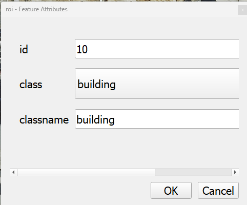
☐ A menu will popup to add attributes. Add a unique id, the class type, and the name of the class in classname. (The classname attribute isn’t used in the analysis, so you can use any notes here.)
☐ To remove polygons, you can open the attribute field and delete rows or modify them. If you’ve made any mistakes, you can remove it from the attribute table or toggle editing off and on.
☐ Once you’re ready to save the layer, click the save button, and then click the Toggle Editing button.
Classifying using Training
The dzetsaka plugin supports several algorithms for classifying the data.
Normally, a supervised classification analysis would be an iterative, cyclical process where training results would be evaluated and then used to refine the training data so that each pass gets closer to having fewer errors in the dataset.
NOTE: This step can take a LONG time to run. Depending on the size of your data, the algorithm chosen, and the speed of your computer.

☐ To run a classification, go to Plugins > dzetsaka and open the Classification dock.
☐ The first box, image to classify, is your raster image (oc6i0…)
☐ The second box, Your ROI, is the Regions of Interest shapefile (roi.shp). Be sure that you’ve saved and stopped editing the file.
☐ The third box, “Column name where class number is stored”, is Class.
☐ The fourth box is the name of the output raster. Click on the three dots button to choose a folder and label an output file name.
☐ Click on the Settings button to choose a Classifer. Gaussian may be the fastest classifier.
☐ When ready, click “Perform the classification”
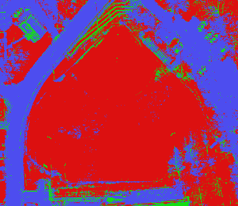
When the output finishes, you should see a raster with a range of values equal to the number of classes that you chose. The raster value is equivalent to the class attribute value in the roi shapefile.
☐ To view the values separately, right-click and go to Properties, and under Symbology, change the Render type to Paletted / Unique Values, and then click Classify.

Evaluating the output from the tutorial data, it hasn’t done a bad job, although there are some obvious problems:
- It’s overestimated roads and to some extent fields. This may be due to roads having tree coverage or roads having pixel colors similar to buildings. Using a dataset with more bands (infrared, uv) might provide better classification, but would also likely reduce the resolution of the results.
- It looks like it’s underestimated buildings, likely for the same reasons above.
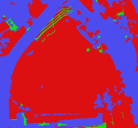
- Overall, there’s a lot of noise – pixels of one type sprinkled in among pixels of other types. To produce a workable output, we’ll smooth the data, and then convert to vector.
This is a first pass at classification. It would make sense, then, at this point to revisit our training data and run the process again.
Smoothing and Vectorizing the Results
Smoothing the Results
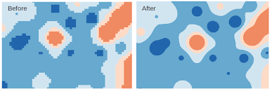
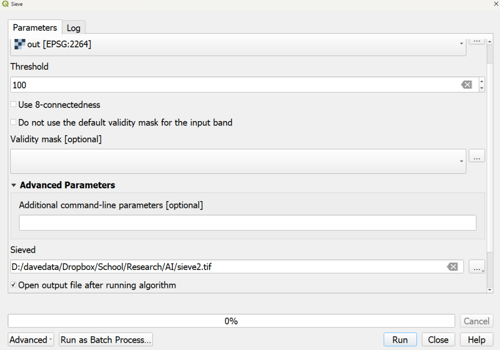
It’s normal to have some noise in the output from your classification. To help smooth the data, we can use the Raster Analysis > Sieve tool in the Processing Toolbox. If you can’t see the Processing Toolbox, go to View > Panels > Processing Toolbox.
Raster smoothing is the process of using neighbors of pixels to smooth values between data. It’s similar to the process that video streaming data uses to “smooth” video when network lags occur. Outlier pixels can be smoothed by choosing from the majority groups of neighbors.
☐ Open the Raster analysis > Sieve tool.
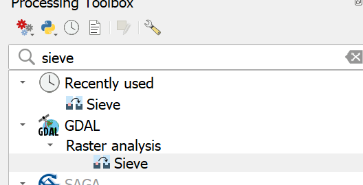
☐ For the input layer, choose the output raster from your classification step.
☐ The Threshold is the number of pixels to be removed. For a noisy dataset, you will need to set this very high – perhaps 100 or higher. This is quite high – fixing the training data and rerunning the classification will also improve this problem.
☐ Set the output file to a new raster.
If you compare the output from sieve to the output from the classifier, you should see a clear difference in noise.
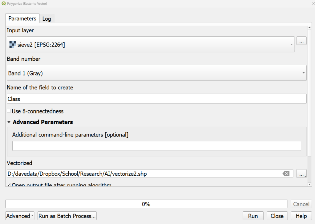
Vectorizing the Results
Finally, we can convert the data to a vector, which allows us to edit the data, remove errors, and then use to retrain the data.
☐ To Rasterize, go to Raster > Conversion > Polygonize (Raster to Vector)
☐ The input layer will be the output from the Sieve function.
☐ The name of the field to create will be “Class”
☐ The vectorized file will be a new shapefile. Run the Polygonize. NOTE: May take a long time!
The results suggest a partial success – let’s evaluate the model and think about next steps.
Validating the Model
Note that there are plenty of limitations with our model and classification.
First, this is a site-specific, time-specific, non-generalized classification method. Different images, locations, or time-periods will require retraining.
Confusion Matrix
To validate the model, we have several options. One is a confusion matrix, which involves comparing regions of a known class and comparing them with what the classifier defined them as:

Confidence Map
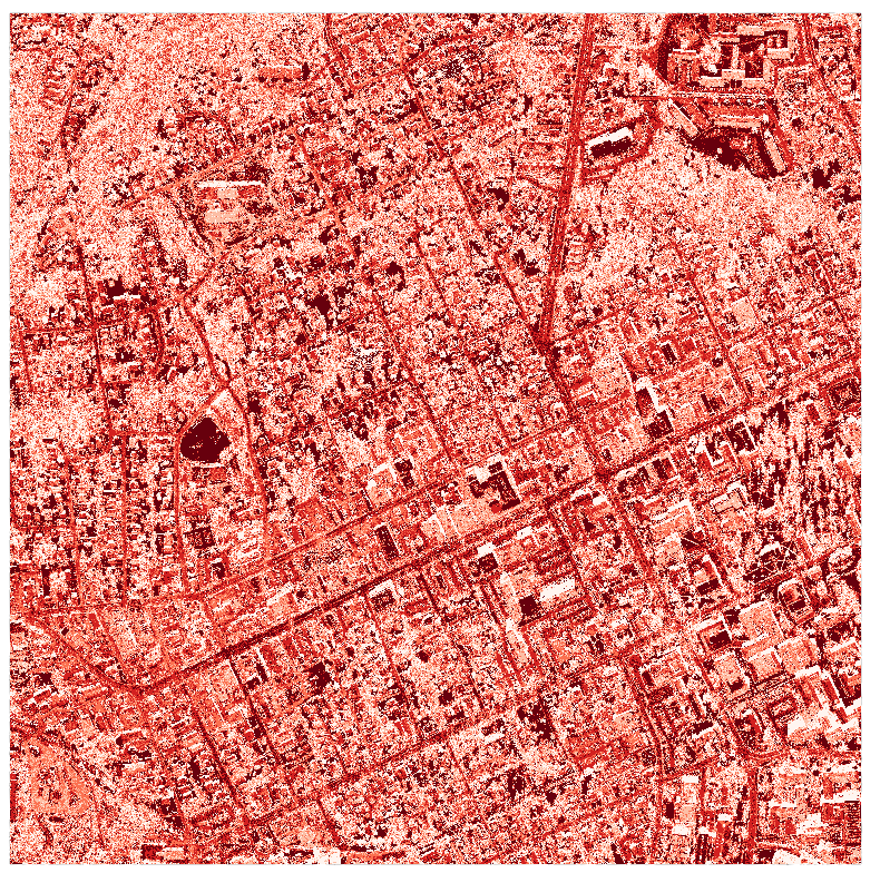
Djetsaka will generate a confidence map, which is how confident the classifier appears to be on a range of 0 to 100% based on the training data for each pixel. This doesn’t meant that the results are valid, only that the output matches the training data. This helps to location potential spatial error in the data.
Cross-Validation
Another technique to test the classifier is cross-validation. This involves comparing the outputs to a known classification – either another dataset or by leaving some of the training data out of the initial learning process.
Overall accuracy can be calculated from the omitted training data by counting the number of pixels in the region that are correctly classified vs. the total number of pixels in the region.
Next Steps
Training and classification of land cover data requires patience and practice. There are plenty of other techniques for image classification available in open source data, including the Semi-Automatic Classification Plugin, used to automatically find and download satellite imagery and process it.
Other software platforms, including ArcGIS, provide pre-made classifiers that can be used for specific purposes.
Once classification has been verified, then using multiple images over time can be used to determine land cover change.
We can determine some critiques of this technique as well, since it requires skill in determining training data, and, as with all AI, Garbage In = Garbage Out. But even basic classification techniques can provide a stepping stone to understanding the landscape and examining change in land.

Leave a comment